About

• What is the difference between modern OpenGL and DirectX?
• Can I make a time-dependend electromagnetic simulation?
• How is a full-screen Windows Modern (Metro) Application different from a desktop OpenGL / DirectX application?

Mathematics

$$\vec{F}=q(\vec{E} + \vec{v}\times\vec{B})$$ Lorentz Force Law for a point charge in an electric and a magnetic field

$$\vec{F}=m\vec{a}$$ Newton's Second Law

$$\vec{E(r)}=\frac{1}{4\pi\epsilon_0}\sum\limits_{i}\frac{q_i}{R^2}\hat{R}$$ The steady-state electric field at \(r\) given \(\vec{R}\) (the vector from a point charge to your point \(r\)) summed over all particles.

$$\vec{B(r)}=\frac{\mu_0}{4\pi}\sum\limits_{i}\frac{q_i\vec{v_i}\times\hat{R_i}}{R_i^2}$$ The steady-state magnetic field at \(r\) given \(\vec{R}\), summed over all particles.

However, these approximates above don't account for the time that it takes for changes in a particle's position to be visible to other particles, because information only travels at the speed of light. These approximate equations above are only correct for non-relativistic, steady-state situations.

For this simulation, I used a (less approximate) equation from my E&M course and stored the history of each particle's motion so that time effects could be properly considered. By setting \(\vec{u}=c\hat{R}-\vec{v}\), the following equations were used:

$$\vec{E(r,t)}=\frac{1}{4\pi\epsilon_0}\sum\limits_{i}\frac{q_iR_i}{(\vec{R_i}\cdot\vec{u_i})^3}((c^2-v_i^2)\vec{u_i}+\vec{R_i}\times(\vec{u_i}\times\vec{a_i}))$$ An updated electric field equation, but where the vector \(\vec{R}\) accounts for when the particle was given a light speed delay

$$\vec{B(r,t)}=\frac{1}{c}\hat{R}\times\vec{E(r,t)})$$ An updated magnetic field equation, calculated using the updated electric field equation

I didn't add the Abraham-Lorentz force to these equations because the particles spontaneously accelerates when done so, with that level of detail also beyond my level of understanding.

Results

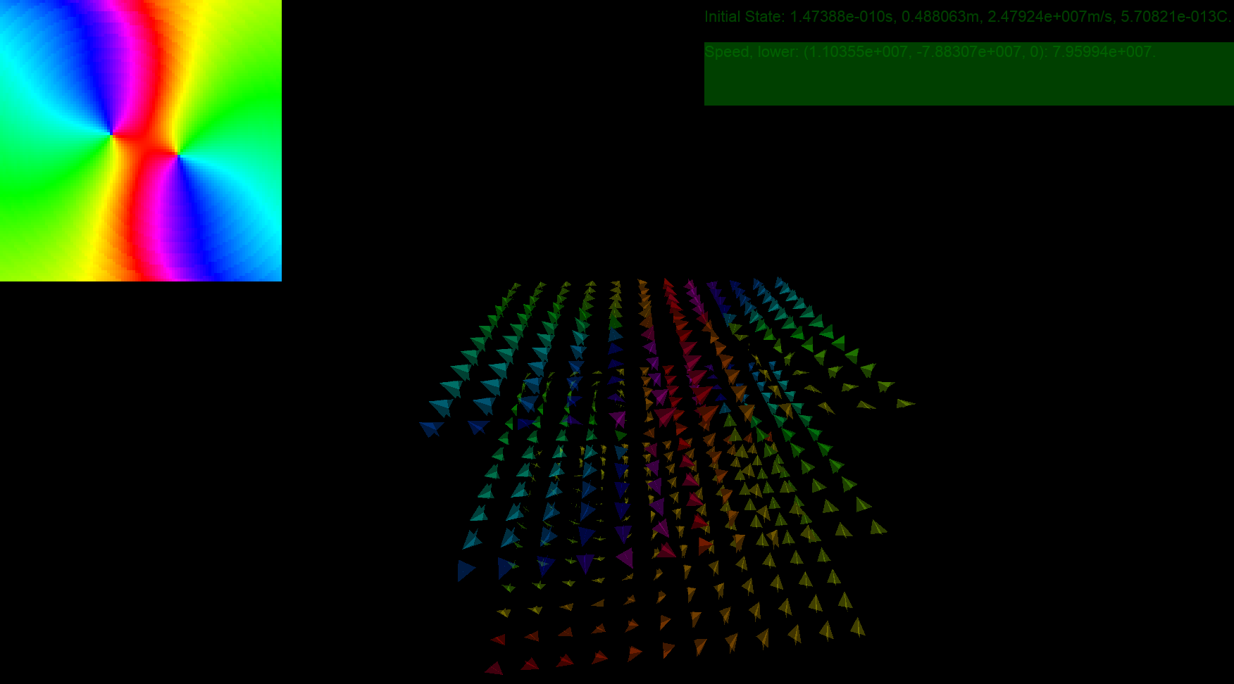
In terms of the software, this screenshot shows:

• Geometry-shader generated arrows
• The usage of both Direct2D and Direct3D to draw info text
• A fullscreen Windows Modern App

In terms of the simulation, this screenshot also shows the electromagnetic waves being propagated over time, as expected.

Surprisingly, I found programming in modern DirectX to be extremely similar to programming in modern OpenGL. In both cases, you:

• Load shaders
• Setup the shader data format
• Load a vertex buffer with triangles
• Batch render through the shaders